Flow of Navier-Stokes fluid past a circular obstacle

\[\begin{split} \mathbb{S}_{\mathbf{u},p} \begin{cases} \Omega = \{(x,y)~:~x^2 + y^2 > R^2~,~|x|<\tfrac{1}{2}L_x~,~|y|<\tfrac{1}{2}L_y\} \\ \partial\Omega_{\text{obstable}} = \{(x,y)~:~x^2 + y^2 = R^2\} \\ \partial\Omega_{\text{left}} = \{(x,y)~:~x=-\tfrac{1}{2}L_x\} \\ \partial\Omega_{\text{right}} = \{(x,y)~:~x=\tfrac{1}{2}L_x\} \\ \partial\Omega_{\text{lower}} = \{(x,y)~:~y=-\tfrac{1}{2}L_y\} \\ \partial\Omega_{\text{upper}} = \{(x,y)~:~y=\tfrac{1}{2}L_y\} \\ \textbf{u}_{\text{E}}\vert_{\partial\Omega_{\text{lower}}\cup\partial\Omega_{\text{upper}}\cup\Omega_{\text{obstable}}}=\textbf{0} & \text{no-flow on other boundaries} \\ \boldsymbol{\tau}_{\text{N}}\vert_{\partial\Omega_{\text{left}}} = p_\text{in}\textbf{e}_x & \text{high pressure on left boundary} \\ \boldsymbol{\tau}_{\text{N}}\vert_{\partial\Omega_{\text{left}}} = \textbf{0} & \text{low pressure on right boundary}\\ \end{cases} \end{split}\]

from lucifex.fdm import FE, CN
from lucifex.sim import run
from lucifex.plt import plot_mesh, plot_colormap, plot_contours, plot_line, save_figure
from lucifex.utils.fenicsx_utils import extract_component_functions
from py.F31_navier_stokes_obstacle import navier_stokes_circle_obstacle

Lx = 2.0
Ly = 1.0
r = Ly / 5
simulation = navier_stokes_circle_obstacle(
    Lx=Lx,
    Ly=Ly,
    r=r, 
    dx=0.05, 
    rho=1.0,
    mu=1.0,
    p_in=8.0,
    dt_max=0.5,
    dt_min=0.0,
    dt_courant=1.0,
    ns_scheme='ipcs',
    D_adv=FE,
    D_visc=CN,
    streamfunction=True,
)

n_stop = 20
dt_init = 1e-6
n_init = 5
run(simulation, n_stop=n_stop, dt_init=dt_init, n_init=n_init)

u, p, psi = simulation['u', 'p', 'psi']
mesh = u.function_space.mesh

time_index = -1
u_n = u.series[time_index]
p_n = p.series[time_index]
psi_n = psi.series[time_index]

ux_n, uy_n = extract_component_functions(('P', 1), u_n, names=('ux', 'uy'))

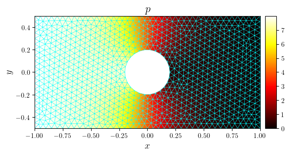
fig, ax = plot_colormap(p_n, title='$p$')
plot_mesh(fig, ax, mesh, color='cyan', linewidth=0.5)
save_figure('p(x,y)_mesh')(fig)

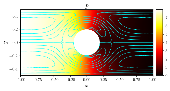
fig, ax = plot_colormap(p_n, title='$p$')
plot_contours(fig, ax, psi_n, colors='cyan', levels=10)
save_figure('p(x,y)_streamlines', thumbnail=True)(fig)

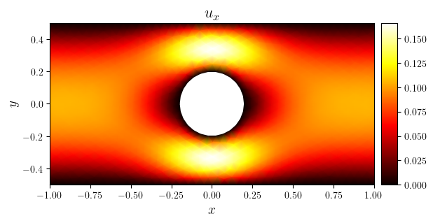
fig, ax = plot_colormap(ux_n, title='$u_x$')
save_figure('ux(x,y)')(fig)

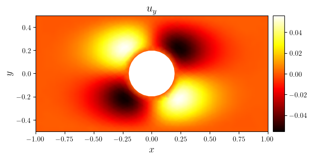
fig, ax = plot_colormap(uy_n, title='$u_y$')
save_figure('uy(x,y)')(fig)

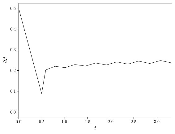
dt = simulation['dt']

fig ,ax = plot_line(
    (dt.time_series, dt.value_series),
    x_label='$t$',
    y_label='$\Delta t$',
)